Terminal unit demodulator design is interesting. A TU must deal with the vagaries of HF radio such as variable noise level, fading, and selective fading. A lot has been written over the years suggesting the best way to demodulate FSK (see TU References). Tests of various demodulators were done (see TU Comparison). These notes are used to inform the design of a DSP-based terminal unit. The DSP-based terminal unit uses DSP techniques to duplicate the design of analog terminal units.
RTTY seems like a great opportunity to learn a bit about digital signal processing. I decided to use the PIC32MZ series of chips since I was most familiar with them. The last 15 years of my career involved work with the PIC32MX.
The Terminal Unit consists of a modulator and a demodulator. The modulator seems like the simplest part while the demoduator is more complex and needs to deal with noise, interference, and selective fading.
The LTSPICE file used in the following tests is here.
FSK can be viewed as an FM signal (generated by frequency modulating an oscillator with the keying signal), or as two Amplitude Shift Keyed signals. FM is typically demodulated by having a limiter (clipper) in the signal path followed by some sort of frequency discriminator (such as a quadrature detector or a PLL). With AM demodulation, there would be no limiter, just tone filters and amplitude detectors. The simplest AM demodulator would just be two filters followed by envelope detectors and low pass filters. Whichever signal (mark or space) was higher would key the loop. However, due to filtering, the mark to space transition is often slow. If the tones are not equal level, bias distortion is introduced. This can be corrected for using Dynamic Threshold Control where the threshold is adjusted based on the latest mark and space envelope detector levels. But, if the data is slow (hand typed), the space may not be frequent enough to make adequate threshold adjustment. This is especially the case with analog circuitry where capacitors are used to hold the envelope levels used to determine the threshold level. However, in the DSP-based terminal unit, memory could hold the space level as long as required. A simple method might be to save an average of the envelope level for mark when the slicer has determined the signal is mark, and the average of the envelope level for space when the slicer has determined the signal is space. The threshold would be the average of the two envelope values (with mark being positive and space being negative). The threshold would be adjusted on a bit by bit basis. This is similar to a method I used to record data on a Stringy Floppy many years ago. In that system, I used the time between transitions to determine if a bit was mark or space. There was an initial value for the threshold time, but each time a bit was received, the threshold was adjusted based on the duration of the bit.
One way to guarantee equal tone levels, even with selective fading, is to limit or clip the signal before it hits the tone filter. At this point, the tone filters and envelope detectors form a frequency demodulator. I have often heard of the "capture effect" of FM. It appears this is due to the limiter.
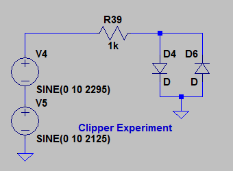
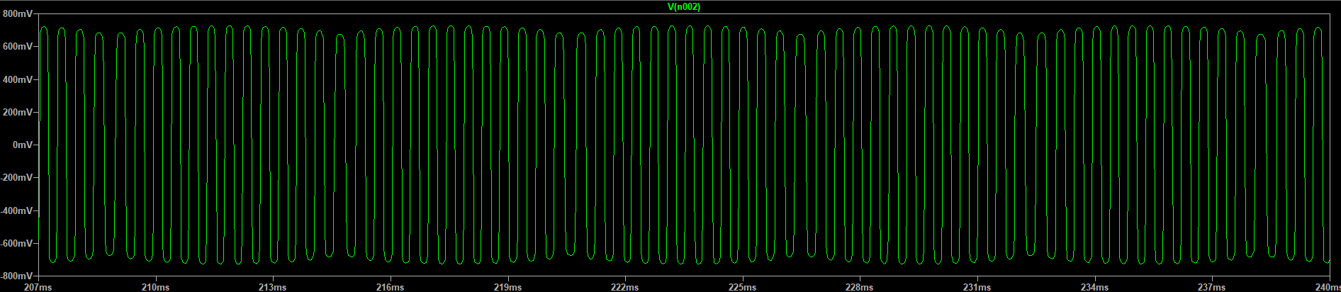
To test "capture effect," the circuit below was simulated in LTSPICE. A 2125 Hz signal and a 2295 Hz signal are added and drive a clipper. The resulting waveform is below.
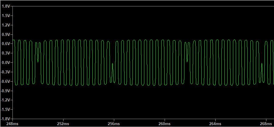
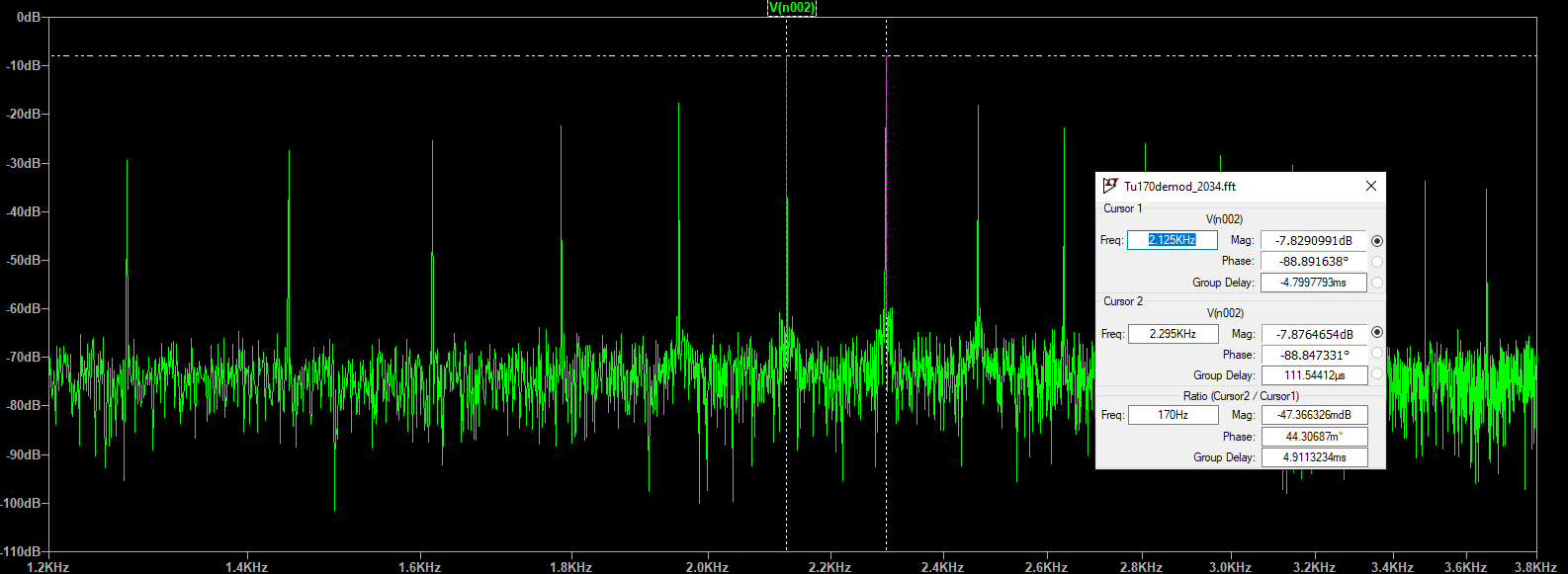
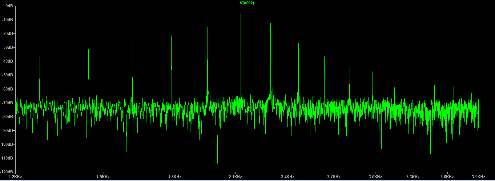
The FFT spectrum view of the clipped signal is below. There are a lot of harmonic and intermod peaks, but the highest peaks are the original tone frequencies. The cursors are set_error_handler on these two peaks. They have about the same level.
Next, the 2295 Hz tone was reduced 3 dB. The resulting clipper waveform and FFT are shown below. 2125 Hz is at -5.4 dB while 2295 Hz is at -12 dB. A 3 dB tone difference into the clipper gives a 6.6 dB difference on the clipper output.
Finally, the level of the 2295 Hz source was increased to values shown in the table below, and the tone levels out of the clipper as measured using the LTSPICE FFT measured.
| 2125 Hz Level Volts | 2295 Hz Level Volts | Clipper Input Tone Difference dB | Clipper Output Tone Difference dB |
|---|---|---|---|
| 10 | 10 | 0 | 0 |
| 10 | 11.22 | 1 | 3 |
| 10 | 12.59 | 2 | 5 |
| 10 | 14.13 | 3 | 6.7 |
| 10 | 15.85 | 4 | 8.2 |
| 10 | 17.78 | 5 | 9.5 |
| 10 | 20 | 6 | 10.9 |
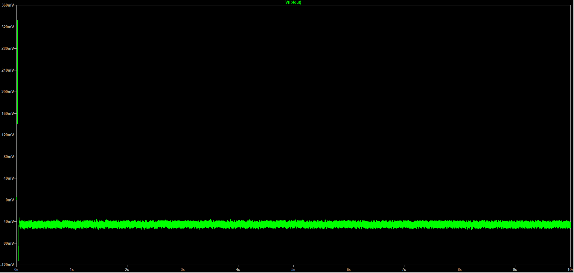
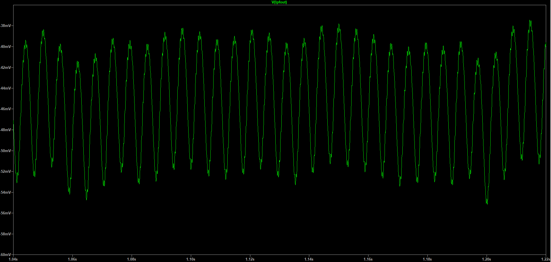
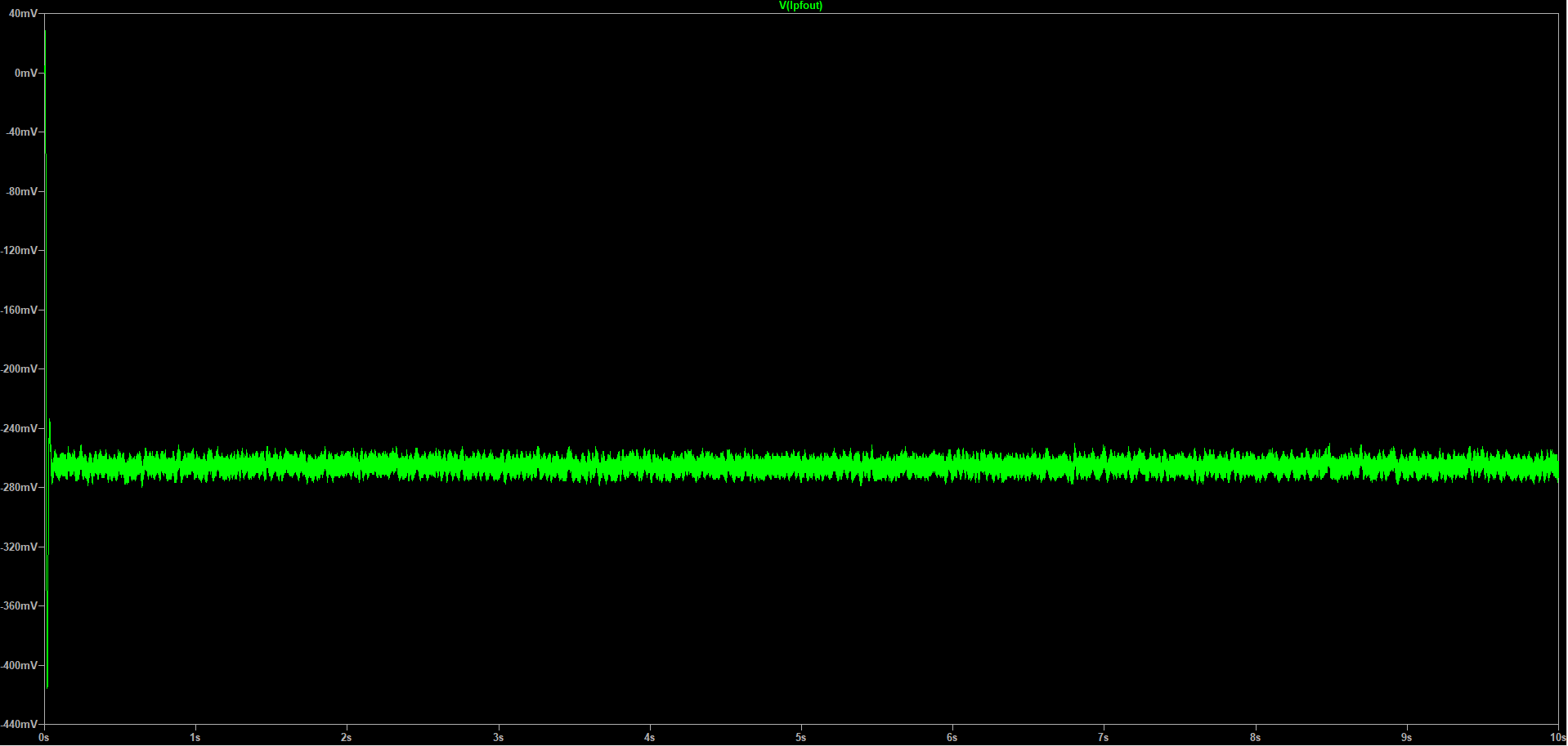
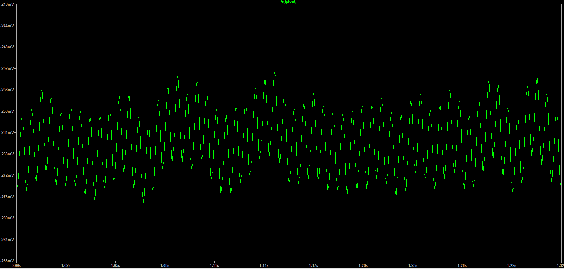
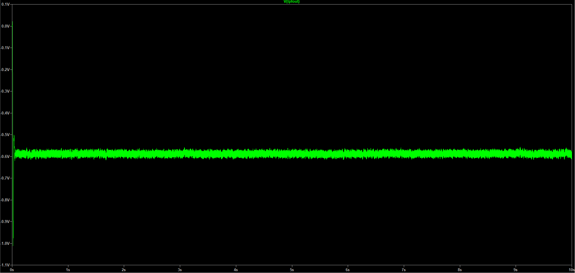
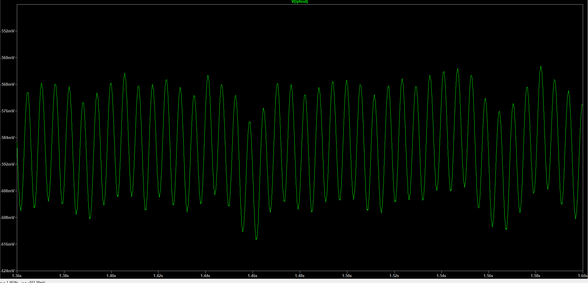
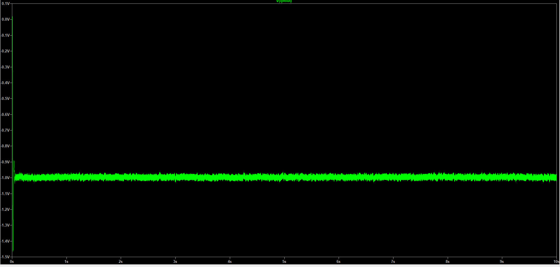
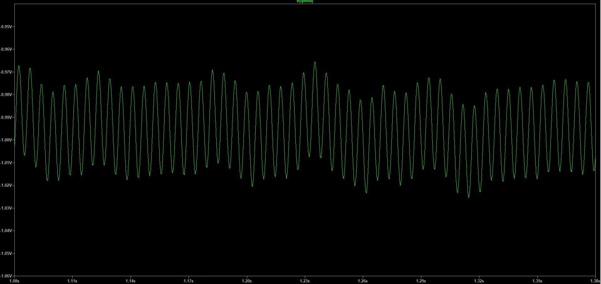
The table above uses levels reported by the FFT in LTSPICE. As suggested in New Horizons in Amateur HF-RTTY Transmission, noise causes instantaneous frequency variations in the limiter output. The article suggests that following the limiter with a bandpass filter would attenuate these variations. However, if they are indeed short, the low pass filter after our discriminator could reduce the effect of the noise. As a test, the TU-170 spice model was driven with two tones (2125 Hz and 2295 Hz) at various levels and the output of the data LPF observed. The mark voltage into the limiter was held at 10V and the space voltage adjusted.
| Space Voltage | dB above Mark | LPF Output | |
|---|---|---|---|
| 10 V | 0 dB | -42 mV 10 second waveform, 180 ms waveform | |
| 11 V | 0.282 dB | -265 mV 10 second waveform, 33 ms waveform | |
| 12 V | 1.584 dB | -580 mV 10 second waveform, 240 ms waveform | |
| 13 V | 2.279 dB | -1.0 V 10 second waveform, 300 ms waveform |
A limiter before the tone filters can guarantee the tone filter outputs are the same in the presence of selective fading. It is further desirable to band limit the signal before the limiter to reduce noise. However, depending on the bandwidth or Q, this filter will "ring" to limit the rise and fall times of the tones. With the rise and fall times being the same, no bias distortion is introduced when the tone levels are compared. However, with selective fading (say a lower level of the tone that is about to start), the ending higher level tone has to fall farther to allow the lower level starting tone to "capture" the limiter. This lengthens the ending tone and shortens the starting tone, introducing bias distortion. As shown in the TU Comparison, some terminal units use limiters, and some do not. Further, those with limiters may not have a bandpass filter in front of the limiter (TU-170) or may have a broad filter (260 Hz in HAL ST-6, 470 Hz in HAL ST-8000).
This problem is discussed in A New Approach to TU Design Using A Limiterless Two-Tone Method. In the circuit, the top filter and envelope detector (using D1) provides a negative voltage to the data LPF (left side of 220k resistor), while the bottom filter and envelope detector (using D4) provides a positive voltage to the LPF. Looking at the bottom filter, D3, the 2M resistor, and the 0.47 uF capacitor develops a voltage proportional to the tone level, but is one half that developed with D4 since the first circuit only uses half the transformer winding. Further, this voltage is subtracted from the positive voltage developed by D4. D3 develops a "slideback" voltage that is proportional to the long term average of the tone amplitude, This voltage is subtracted from the instaneous voltage developed by D4 and the .002 uF capacitor. The result is that in a selective fade, less "slideback voltage" is subtracted from the instaneous envelope value resulting an a relatively constant voltage to the LPF when the tone is present, even if the tone is fading.
An expriment was run on the LTSPICE simulation of the Flesher TU-170. The simulation was run with 20.8 dB selective fading (space 20.8 dB below mark) with and without white noise, and with and without a bandpass filter in front of the limiter.
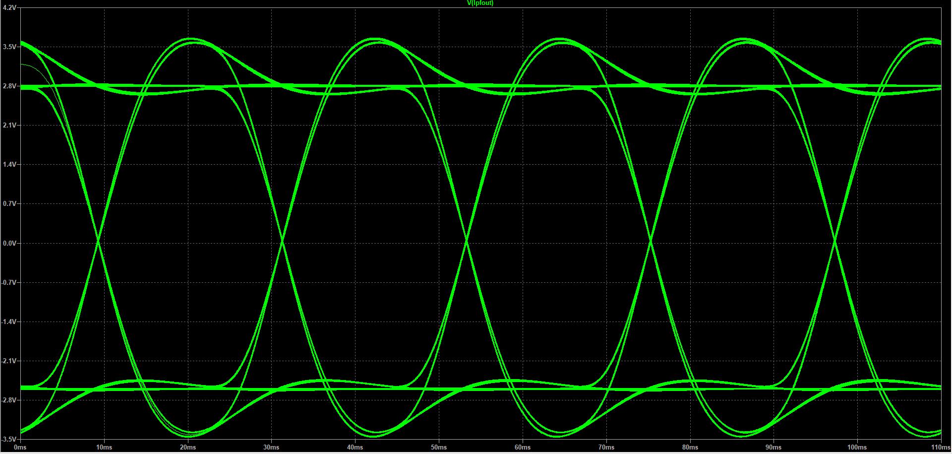
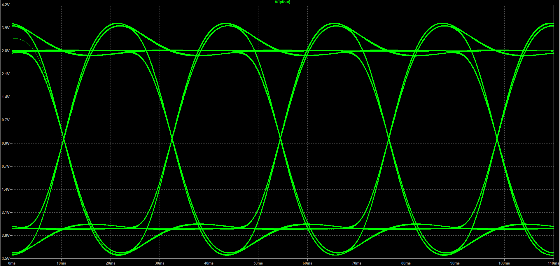
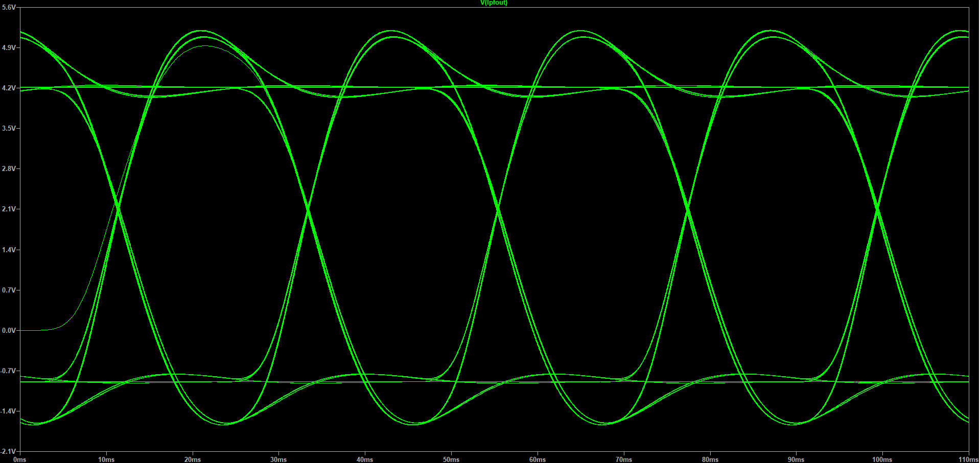
The image below is the eye diagram with 20.8 dB selective fading and no filter in front of the limiter. Note that the crossover points are at zero volts.
The image below is the eye diagram with 20.8 dB selective fading and a 2 pole BPF with FC = 2208.365 Hz with Q = 10, Bandwidth = 220.8 Hz. Note that the crossover point has moved up to
129 mV. If we keep the threshold at 0.0 V, a bit length varies between 21.2 ms and 22.03 ms. Not bad.
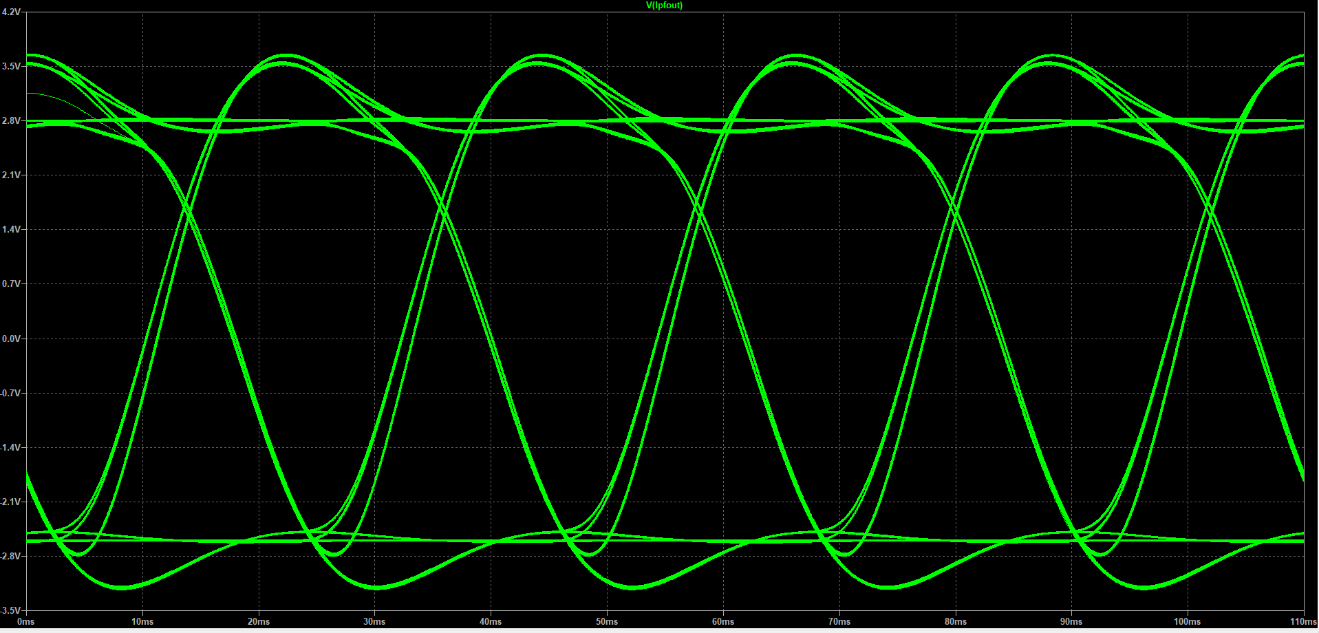
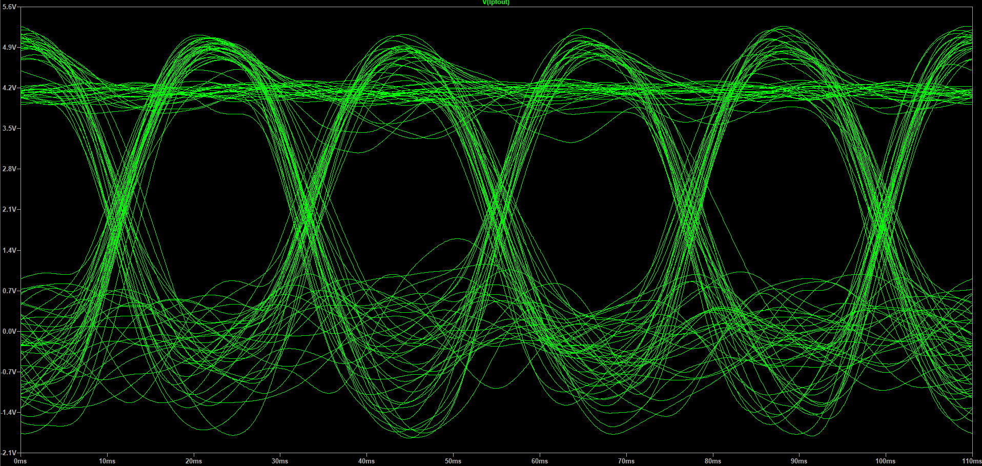
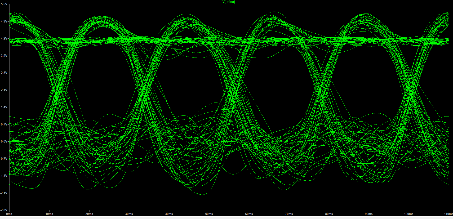
The image below is the eye diagram with 20.8 dB selective fading and a 2 pole BPF with FC = 2208.365 Hz with Q = 20, Bandwidth = 110.4 Hz. Note that the crossover points are now about 1.7 V. The time of a bit varies from 14 ms to 29 ms if the threshold remains at 0V. This is the issue identified in A New Approach to TU Design Using a Limiterless Two-Tone Method. As noted at RTTY Terminal Unit Comparison, Flesher TU-170 has a limiter and no filter in front of it. Also, the HAl ST-8000 can be operated with a limiter and a pre-limiter BPF with Q = 4.7.
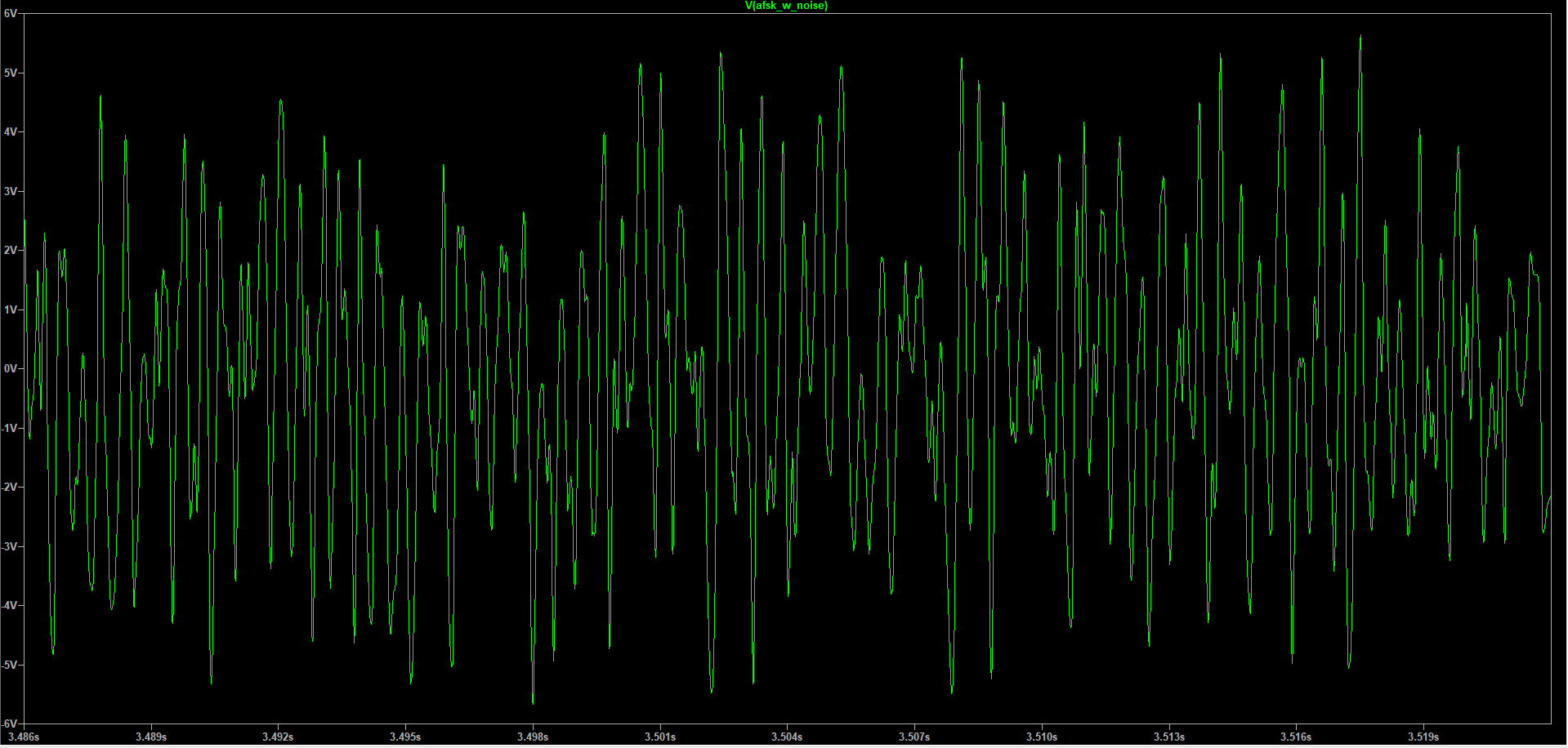
The spice file for the above tests is here. Note that an open loop op amp acting as an analog comparator is used as the limiter. Wires can be moved around to use different pre-limiter filters. Resistors can be changed to insert noise into the AFSK signal. V3 can be changed to change the amount of selective fading.
Though a filter before the limiter reduces noise at the limiter, the eye diagram does not really look any better in the presence of selective fading.
The change from 850 Hz shift to 170 Hz shift has reduced the effects of selective fading (now both tones tend to fade together without large level difference). This may reduce the bias distortion introduced by placing a filter before the limiter. Note that the Flesher TU-170 (see also LTSPICE analysis) uses a limiter in front of the tone filters and does not have a filter before the limiter.
In the DSP TU, it would be interesting to try several approaches.
Looking at the HAL ST-8000, we find four slectrable bandpass filters in front of the limiter. The limiter is a 709 op amp running open loop (as a voltage comparator). The ST 800 also offers an AGC instead of a limiter. This would be used with dynamic threshold control.
According to Filters for RTTY, a close approximation of the ideal filter for the tone bandpass filter is a 3 pole Butterworth filter with a bandwidth of 1.2 times the baud rate. Each tone is amplitued modulated with the data (mark tone amplitude is 100% during mark and 0% during space). The data is a varying frequency square wave with the highest frequency being 22.72727 Hz (1 /2*BitTime where BitTime is 22 ms). This highest frequency is when there are alternate mark and space where the signal is low (space) for 22 ms and high (mark) for 22 ms, giving a period of 44 ms. 1.2 times the baud rate of 45.45455 yields a suggested bandwidth of 54.54545 Hz. A square wave consists of the fundamental (22.72727 Hz) plus odd harmonics. The third harmonic would be at 68.18182 Hz. Since amplitude modulation produces two sidebands, one below and one above the carrier, a 22.72727 Hz sine wave would produce two sidebands that are 45.45455 Hz apart (the same as the baud rate). The 54.54545 Hz bandwidth passes the sideband of the fundamental but attenuates the sidebands due to the harmonics of the keying signal.
The tone bandpass filters act as a low pass filter on the sidebands (attenuating the sidebands that are farther from the tone frequency - the carrier). As such, it would be interesting to see how this attenuation affects the rise time of the envelope. For a single pole filter, rise time is about 0.35/FH. Since the bandwidth of the tone BPF is 1.2 times the baud rate, the cutoff frequency is 0.6 times the baud rate above and below the tone frequency (not exaclty, since the center frequency of a band pass filter is sqrt(FL*FH), but this is a close approximation). Therefore, the sideband cutoff is 0.6 * 45.45455 Hz = 27.27 Hz. This would yield a rise time of 0.35 / 27.27 Hz = 12.8 ms or about half a bit time.
Filters for RTTY also suggests that the data low pass filter (after the discriminator) should also be a 3 pole butterworth filter with a cutoff frequency of 0.6 times the bit rate. This is slightly above the square wave fundamental of the keying signal. For 45.54545 baud, the suggested cutoff frequency is 27.27273 Hz. Using the rise time formula above, this filter would also have a rise time of 12.8 ms.
When rise times are cascaded, the resulting resulting rise time is the square root of the sum of the squares of the individual rise times. Therefore, the combination of the tone bandpass filter and the data LPF would have a rise time of 18.1 ms.
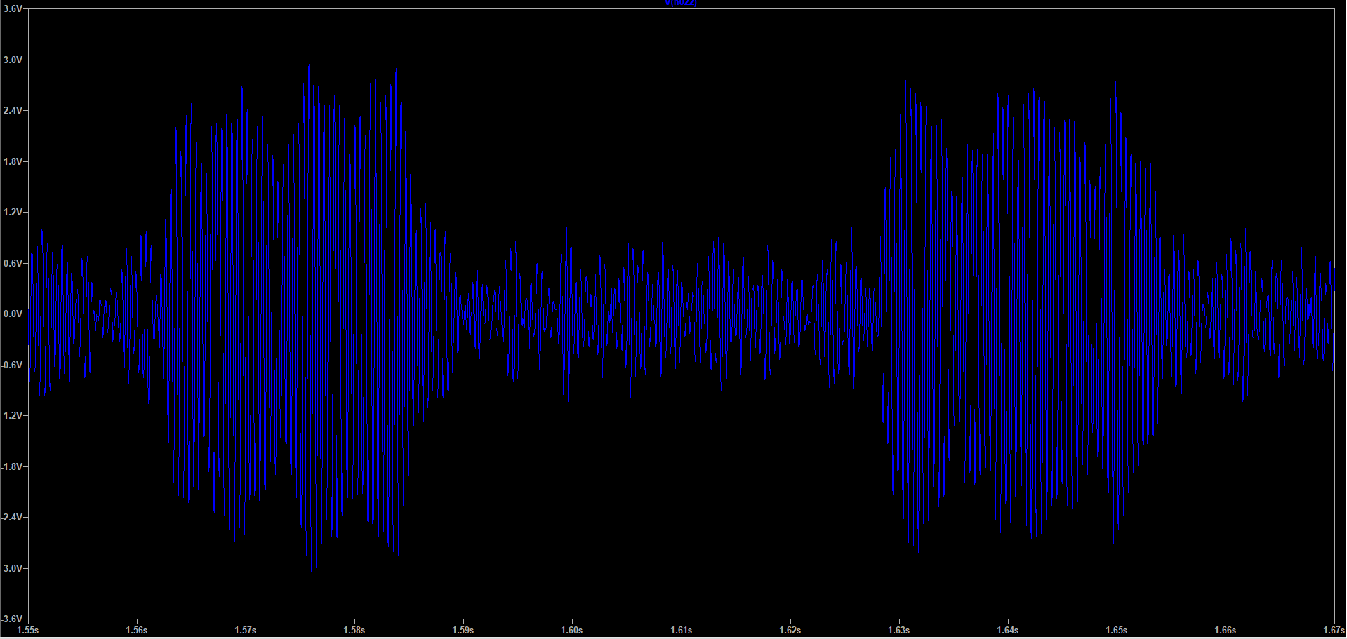
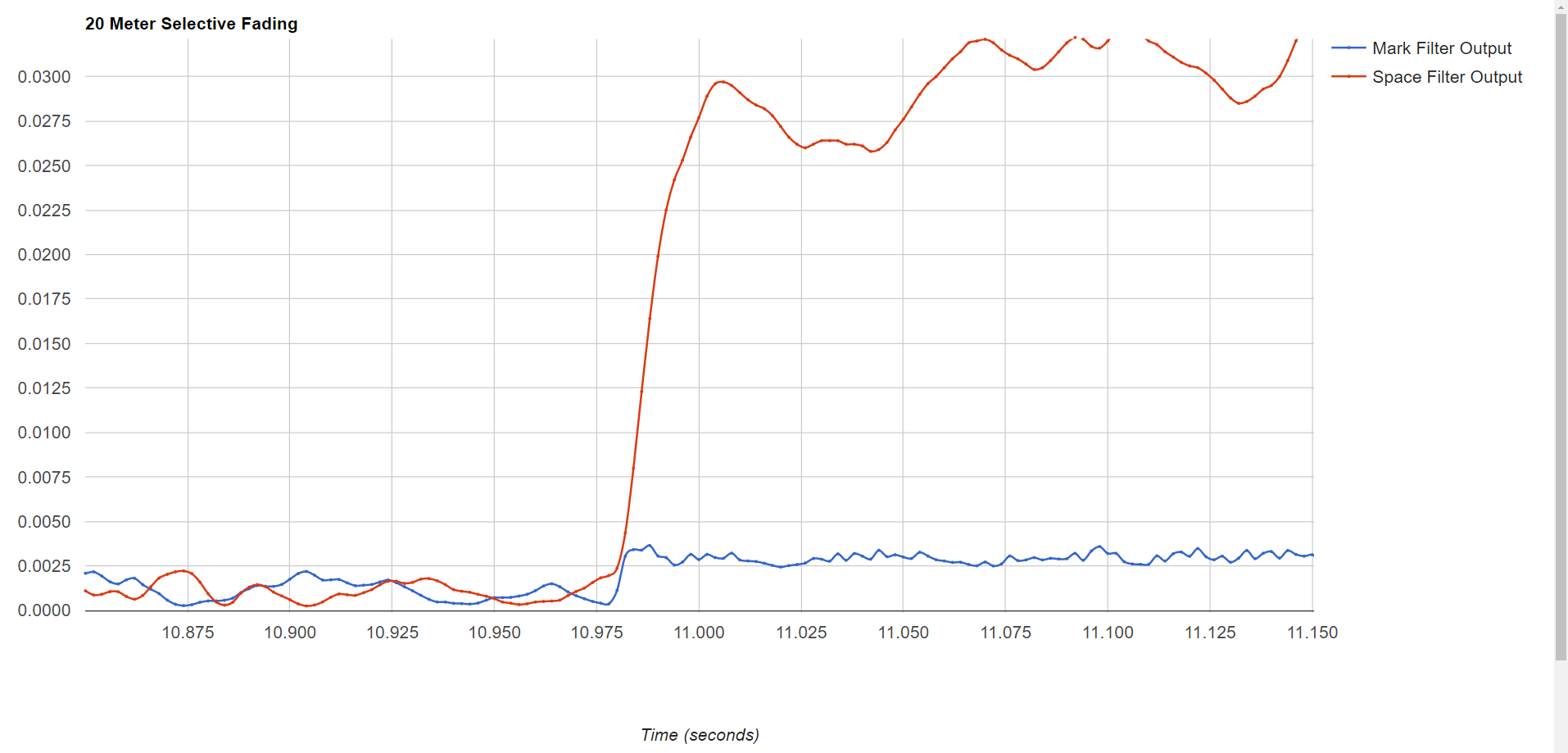
An experiment was run to look at selective fading. Both mark (2125 Hz) and space (2295 Hz) were transmited simultaneously from Tucson AZ at 14.2 MHz USB at 15 watts. The KFS websdr (Half Moon Bay CA) was used to record the tones for 10 minutes. The receiver AGC was turned off so overall fades would be visible. The recorded audio was then run into the start of my DSP TU. The tones were run through biquad bandpass filters with a Q of 50. The filter outputs were run through the absolute value function (full wave rectification) to a two pole low pass filter with a cutoff of 68 Hz. The output of these low pass filters was logged every 2 ms. Below are links to the raw CSV data and graphs of each minute. Drag over an area to zoom in and right click to return to the full minute. Because the test was done USB, the normal frequency inversion did not occur. therefor, the mark signal is at the lower RF frequency (not LSMFT). Zoom into an area by dragging over the area. Return to full scale with a right click. it can take several seconds for the graph to appear, as there is a LOT of data.
In general, both tones fade together, but with a slight time offset (0 to 5 seconds).
Zooming into the time when the first tone starts, we can see the slight mark filter leakage (blue line increasing a bit when the red line increases). Further, it takes about 25 ms for the space filter output to transition to full output.
Another test of 20 meter selective fade was run. Two tones separated by 850 Hz were transmitted on 14.195 MHz USB. The tones were 1075 Hz and 1925 Hz. The old 2125 and 2975 Hz tones were not used because the SSB transmitter severely attenuated the 2975 Hz tone. The signal was received at the KFS websdr. The received audio is here. The data is from the same DSP as above, but the biquad BPFs are tuned to the new tone frequencies. In this particular test, there was very little selective fading. Both tones went up and down nearly simultaneously. The data is listed below.
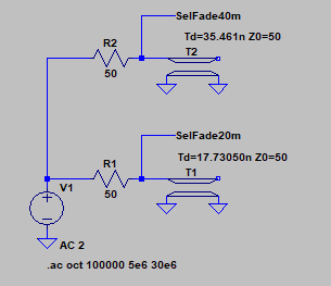
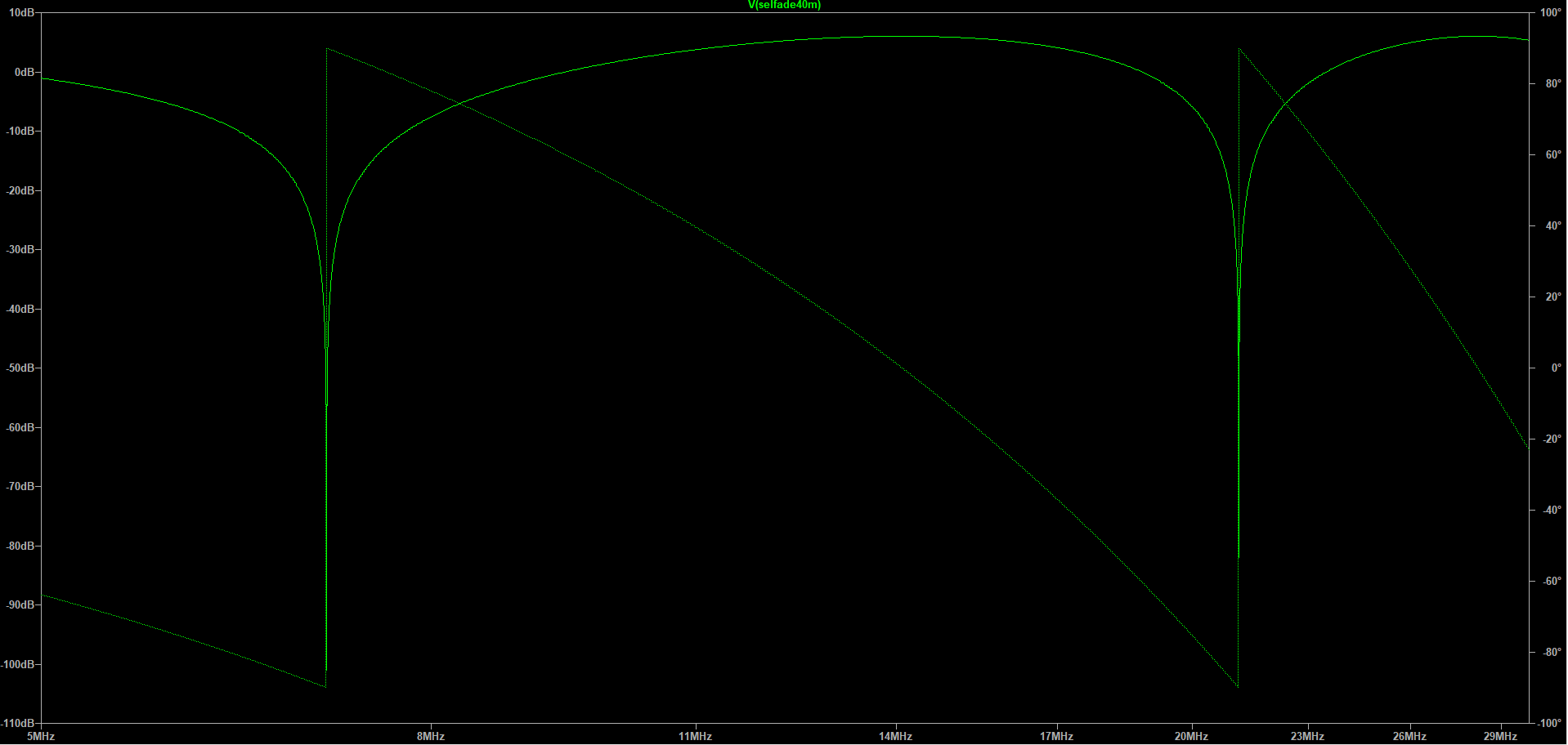
In addition, an LTSPICE simulation of selective fading was done. The LTSPICE file is here. In the circuit below, An AC generator drives a 50 ohm transmission line that is 1/4 wave long at about 14.1 MHz. The signal travels down the line and is reflected from the open end of the line. When the reflection gets back to the 50 ohm resistor driven by the source, the reflection is "added" to the driving signal resulting in a voltage null at that point. This is similar to an ionospheric multipath signal where the signal arrives over two paths with a difference of 35.461 ns with the signal level over both paths being equal. This would be a worst case fade. On the graphs, 0 dB is the level that would be present with no reflection. Outside the null, the level goes above 0 dB as the reflection adds to the original signal instead of cancelling it. To simulate selective fades on both 20 and 40 meters, two transmission lines are used, one for 20 and the other for 40.
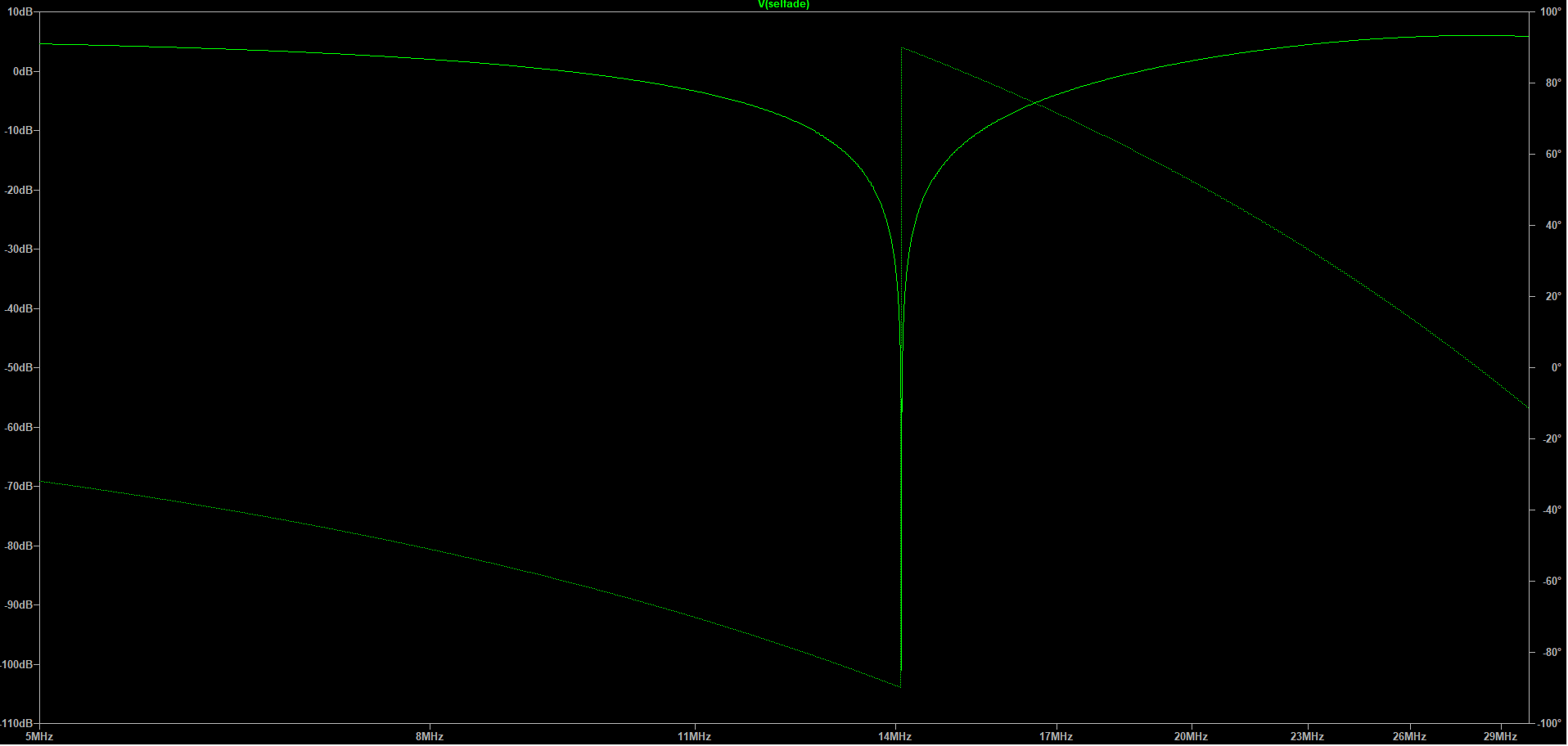
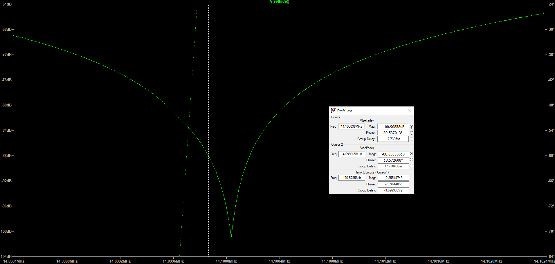

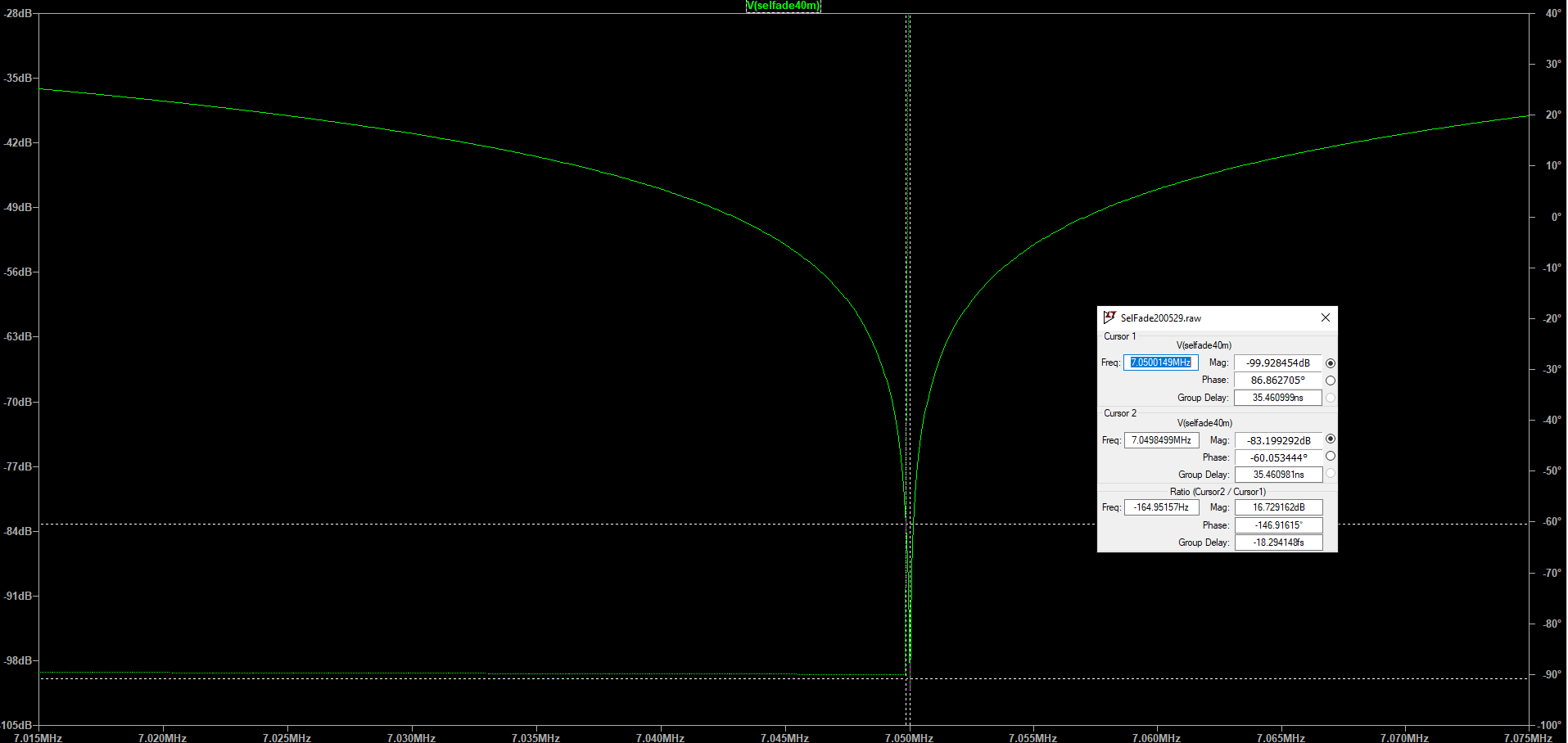
Narrower shift (170 Hz) does reduce the level difference between mark and space in a fade. Both tones tend to fade together (though one will null at one time and the other at another time as the path lengths vary). In a full null, one frequency is down about 101 dB from the level with no multipath, and the other frequency is down 88 dB. In such a case, it is likely that both frequencies would be below the noise level.
However, on 20 meters, with wide shift (850 Hz), one frequency is still down about 101 dB, but the other is down about 75 dB. That 13 dB difference MAY put one of the frequences above the noise and allow copy through the fade (using frequency diversity).
These simulations are a very simple worst case analysis. In actual practice, the signals arriving over the two paths may not have the same amplitude resulting in incomeplete cancellation and a null that is not as deep. The graphs in the previous section show actual selective fading over a 10 minute period. It appears that in that 10 minute sample, there was no time when both frequencies dropped to the noise level at the same time. However, a wider shift would provide a higher level for the non-nulled frequency.
The DSP TU software allows the audio output (PWM through low pass filter) to be switched to various points in the system. In normal operation, it is connected to the DDS tone generator. It can also be switched to the input ADC, limiter output, each of the tone filter outputs, the mark and space data filter outputs, and the "discriminator output" (mark data filter output minus space data filter output). To test various filter configurations, random AFSK with a 22 ms bit time was generated with LTSPICE. The noise-free AFSK with no selective fading is here. The discriminator output was monitored on a scope with long persistence to generate an eye pattern. The random 22 ms bit time data was used instead of a typical RTTY signal like ITTY because the stop bit is normally 31 ms long. Not having every bit be 22 ms will cause the eye diagram to be corrupted.
TU-170 FiltersThe eye diagram at the right is from a software duplicate of the TU-170. The limiter is implemented using the copysign function. If the output of the ADC (once converted to a double with 0.0 representing mid-scale) is positive, the limiter output is 1.0. If negative, the limiter output is -1.0. This is similar to using an analog comparator as a limiter.The mark and space band pass filters consist of three cascaded biquad bandpass filters, each with a Q of 13. The overall Q is Qn / sqrt (2^(1/n) -1) where Qn is the Q of each filter and n is the number of filters. The overall filter Q is 25.5. The bandwidth of the 2125 Hz filter is 2125/25.5 = 83 Hz. Meaurement of the SPICE model showed a bandwidth of 89 Hz, which is pretty close. Filters for RTTY suggests the ideal tone BPF is a 3 pole filter with a bandwidth of 54.5454 Hz. This filter is 6 pole and a bit wider. Instead of envelope detection followed by a single data filter, each tone is full wave rectified using the absolute value function. The rectified tone then goes to a separate data low pass filter for mark and another for space. The data LPFs have a cutoff frequency of 68 Hz. The output of the mark data LPF minus the output of the space LPF is the "discriminator output" shown at right. | 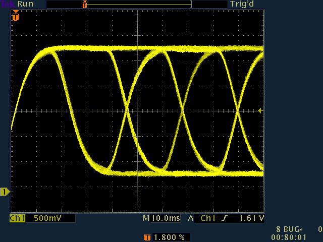 |